3D Residual Encoder U-Net (nnU-Net ResEnc)
From first principles - what U-Net, 3D U-Net, and nnU-Net are and why they matter for medical imaging - through to the ResEnc architecture: a residual encoder with a lightweight convolutional decoder, six stages, [32, 64, 128, 256, 320, 320] features per stage. Full architecture breakdown, published evidence, nnU-Net integration, and from-scratch code.
00 Foundations: what U-Net, nnU-Net, and the residual encoder actually are
This section is written for readers meeting these three terms for the first time - students, clinicians moving into imaging research, or engineers coming from 2D computer vision. If you already know the basics, skip to Section 01.
What "segmentation" means, and why it's different from classification
Image classification answers "what is in this image?" with a single label. Semantic segmentation answers a much harder question: "which class does every single pixel (or, in 3D, every voxel) belong to?" In medical imaging this means producing a mask the same size as the input scan, where each voxel is labeled as, say, liver, tumor, or background. That per-voxel output is what a radiologist or surgeon can actually act on - it gives a volume, a boundary, a shape - not just a yes/no answer.
U-Net (2015): the original idea
U-Net was introduced by Olaf Ronneberger, Philipp Fischer, and Thomas Brox at the University of Freiburg for the 2015 ISBI cell-tracking and neuronal-structure segmentation challenges. At the time, the dominant approach to pixel-wise labeling was a sliding-window classifier: run a small classification network over every possible patch of the image and label the center pixel, one patch at a time. It worked, but it was extremely slow and it treated overlapping patches independently, wasting computation and struggling with limited annotated data.
U-Net's insight was architectural: build a single fully convolutional network shaped like the letter U. A contracting path (encoder) repeatedly applies two 3x3 convolutions plus ReLU, then downsamples with 2x2 max-pooling - this half of the network answers "what is in this image" (context) at progressively coarser resolutions. A mirrored expanding path (decoder) upsamples back to full resolution using transposed convolutions - this half answers "where is it" (localization). The key trick connecting the two: at every resolution level, feature maps from the encoder are copied and concatenated onto the corresponding decoder level, before the convolutions there. These are the skip connections - they hand the decoder back the fine spatial detail that pooling destroyed, so the network doesn't have to reconstruct edges and boundaries from a heavily compressed representation.
The original paper demonstrated the network could be trained end-to-end from very few annotated images - a critical property for medical and biological imaging, where pixel-level ground truth is expensive to produce and datasets are small by computer-vision standards. Heavy data augmentation (elastic deformations in particular) compensated for the limited data. U-Net won the ISBI 2015 cell tracking challenge and became, within a few years, the default starting point for almost every biomedical segmentation task.
3D U-Net (2016): from slices to volumes
The original U-Net operated on 2D images. CT, MRI, and other volumetric modalities are stacks of 2D slices representing one continuous 3D structure, and a purely 2D network processing slice-by-slice cannot see how a structure connects, curves, or changes shape along the axis perpendicular to the slice. Özgün Çiçek, Ahmed Abdulkadir, Soeren Lienkamp, Thomas Brox, and Olaf Ronneberger addressed this directly in 2016 with 3D U-Net: every 2D operation in the original architecture - convolution, pooling, up-convolution - was replaced with its volumetric (3D) counterpart. The network now takes a 3D patch as input and produces a 3D segmentation mask as output, letting it learn spatial patterns across all three axes simultaneously. Their paper's subtitle, "learning dense volumetric segmentation from sparse annotation," also introduced a semi-supervised training setting: the network could learn from volumes where only a handful of 2D slices had been manually annotated, then generalize the segmentation to the full 3D volume.
nnU-Net (2018 / 2021): configuration as the real bottleneck
By the late 2010s, U-Net variants dominated medical image segmentation leaderboards - but every winning submission also carried a bespoke, hand-tuned pipeline: a particular patch size, a particular normalization scheme, a particular loss weighting, chosen by trial and error for that one dataset. Fabian Isensee and colleagues at the German Cancer Research Center (DKFZ) observed that the choice of "novel architecture" mattered far less than getting these mundane pipeline decisions right, and that most published architectural improvements failed to reproduce once compared against a properly-configured U-Net baseline.
nnU-Net ("no-new-Net") is their response: not a new architecture, but a self-configuring framework that inspects a new dataset's image sizes, voxel spacing, intensity distribution, and class balance, then automatically derives the network topology, patch size, batch size, preprocessing, and augmentation policy from a fixed set of rules and heuristics - no manual tuning per dataset. Rather than proposing one clever architecture, nnU-Net trains several candidate configurations (2D, 3D full-resolution, and a low-resolution + cascade variant for very large volumes) and empirically picks the best one, or ensembles them, via cross-validation. First released as a 2018 arXiv preprint and a 2019 conference paper, it was formalized in Isensee et al.'s 2021 Nature Methods paper, where it won 33 of 53 international segmentation-challenge tasks it was evaluated on without any dataset-specific modification - evidence that rigorous, automated configuration was doing more work than architectural novelty.
The residual encoder preset (ResEnc, 2024): where nnU-Net's own baseline improved
Years after the original 2021 result, the same DKFZ group revisited their own baseline. Their 2024 MICCAI paper, nnU-Net Revisited: A Call for Rigorous Validation, re-ran the comparison against newer proposed architectures - transformer-based and Mamba-based models among them - under matched, rigorous conditions (same data splits, same compute budget, same evaluation protocol). The conclusion: once nnU-Net's own convolutional backbone was scaled up - specifically, by replacing its plain convolutional encoder with a residual encoder (borrowing the residual-block design from He et al.'s 2016 ResNet) and giving it more capacity, more GPU memory, and larger patch sizes - it matched or beat most of the newer architectures that had claimed to surpass it. That scaled-up configuration is what's shipped today as the ResEnc presets (M / L / XL) inside nnU-Net v2, and it's the architecture this guide focuses on from Section 03 onward.
Why this line of work matters for medical image processing specifically
- Annotated data is scarce and expensive. Producing a voxel-accurate 3D mask requires an expert (often a radiologist) manually tracing structures across dozens to hundreds of slices. U-Net's data-efficient design and heavy augmentation were built directly around this constraint, unlike architectures developed for natural-image datasets with millions of labeled examples.
- Anatomy is inherently 3D and multi-scale. Organs, vessels, and tumors have shapes and continuity that only make sense in 3D; a network needs both a large receptive field (to recognize an organ) and precise local detail (to trace its boundary) - exactly what the encoder/decoder + skip-connection design provides.
- Datasets vary enormously across institutions, scanners, and modalities. A hand-tuned pipeline optimized for one hospital's CT protocol often fails on another's. nnU-Net's automatic fingerprinting-based configuration directly targets this generalization problem, which is a major practical barrier to clinical deployment.
- Reproducibility has been a real problem in the field. The 2024 ResEnc paper's central finding - that many published "improvements" don't hold up against a properly configured baseline - is itself an important methodological lesson for anyone doing medical imaging research: always compare against a rigorously tuned nnU-Net baseline before claiming a new architecture is better.
01 Why 3D instead of 2D
CT and MRI scans are inherently volumetric - a stack of 2D slices that together encode 3D anatomical structure. Processing slices independently with a 2D network throws away context along the depth (z) axis: a tumor's shape, continuity, and relationship to neighboring structures span multiple slices.
The original 3D U-Net (Cicek et al., 2016) extended the 2D U-Net by replacing every 2D operation (convolution, pooling, up-convolution) with its 3D counterpart, letting the network learn spatial features across all three axes simultaneously.
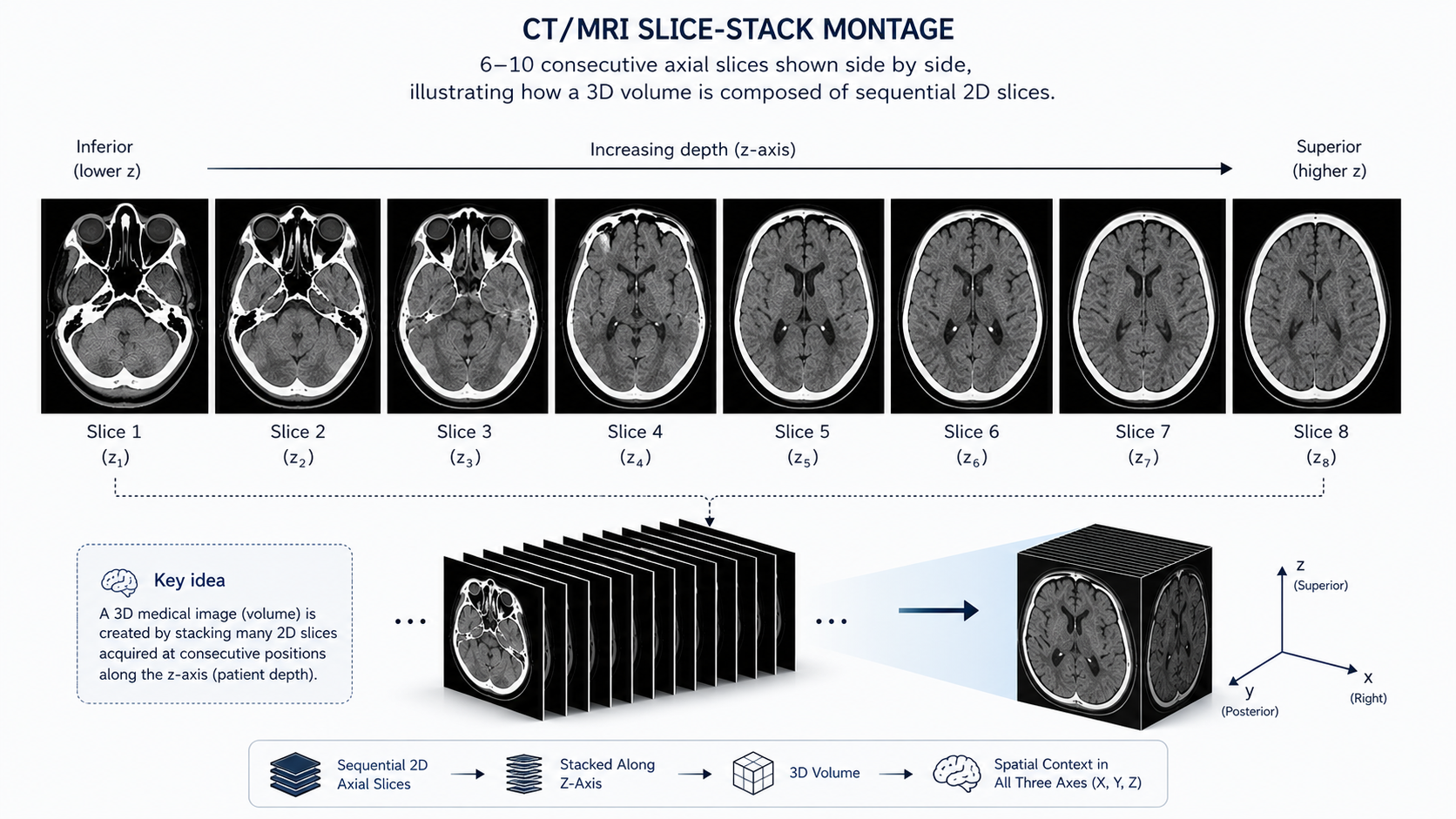
Figure 1: CT/MRI slice-stack montage showing sequential axial 2D slices forming a continuous 3D volume.
02 Encoder / decoder basics
Every U-Net-style network, including the residual-encoder variant covered in this guide, is built from three structural components. The encoder (contracting path) is a stack of convolutional blocks, each followed by downsampling - it captures context, progressively compressing spatial resolution while increasing channel depth. The decoder (expansive path) mirrors the encoder using transposed convolutions to restore spatial resolution - it enables precise localization. Skip connections concatenate encoder feature maps with corresponding decoder feature maps at every resolution level, combining deep semantic context with sharp boundary detail.
What distinguishes the architecture covered in this guide from a vanilla U-Net is where the network spends its capacity: the encoder is made heavier (residual blocks, more blocks per stage as depth increases) while the decoder is kept deliberately light (a single convolution per stage). Section 03 covers this in detail.
03 The ResEnc architecture: residual encoder + lightweight decoder
This guide covers nnU-Net's ResEnc preset: a UNet built with a residual encoder and a lightweight convolutional decoder. The architecture has six stages, with [32, 64, 128, 256, 320, 320] features per stage, respectively. Two design choices define it:
- Residual encoder: every encoder stage is built from residual blocks (two 3x3x3 convolutions with instance normalization and LeakyReLU, plus an identity/projection skip added back before the final activation), rather than plain stacked convolutions. This is where the network's representational capacity is concentrated, and deeper stages typically stack more residual blocks than shallow ones.
- Lightweight decoder: each decoder stage uses a single plain convolution block (no residual connections) after upsampling, rather than mirroring the encoder's residual blocks. Since the decoder's job is mostly to relocate and refine features the encoder already extracted (helped heavily by the skip connections), it doesn't need the same capacity, which keeps compute and memory cost down without hurting accuracy much.
- Capped channel width: channels grow stage over stage (32 to 64 to 128 to 256) but are capped at 320 for the last two stages, rather than continuing to double indefinitely. This keeps the deepest, most expensive layers of the network from growing without bound.
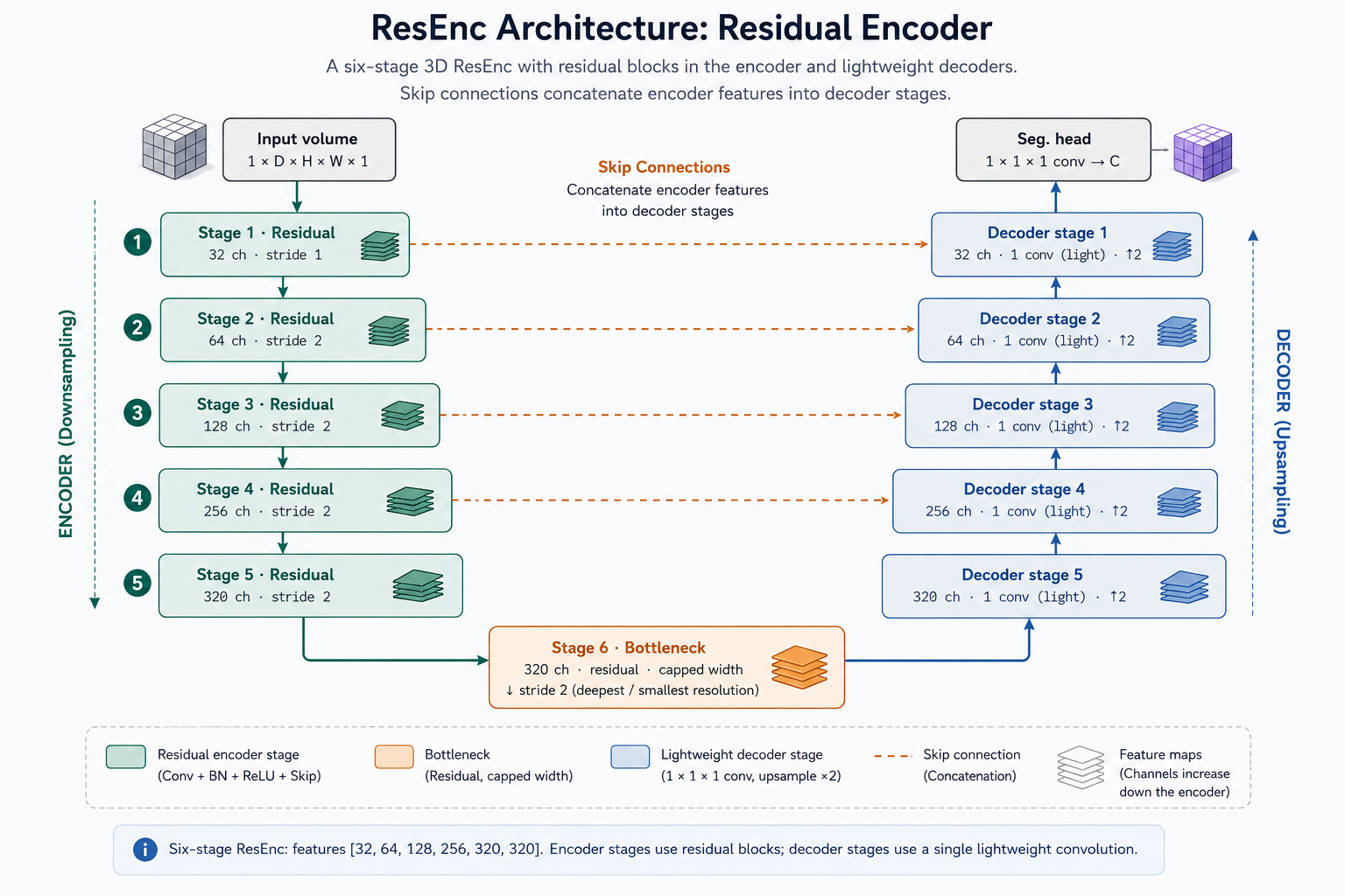
Figure 2: 3D Residual Encoder U-Net (ResEnc) Architecture diagram showing six-stage residual encoder, bottleneck, and lightweight five-stage decoder with skip connections.
What's inside a residual encoder block
Each residual block in the encoder follows the standard pre-activation-style residual pattern used throughout nnU-Net's ResEnc presets: two 3x3x3 convolutions (each followed by instance normalization and LeakyReLU), with the block's input added back to the output before the final activation. When the stage downsamples or changes channel count, the skip path uses a strided 1x1x1 convolution to match shape before the addition.
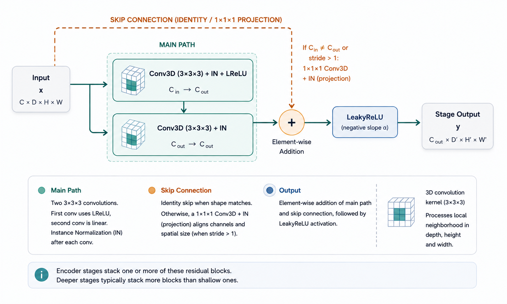
Figure 3: Internal structure of a single residual encoder block showing two convolutions on the main path and identity/projection skip connection.
Stage-by-stage summary
| Stage | Features | Encoder block | Decoder block | Spatial change |
|---|---|---|---|---|
| 1 | 32 | Residual (×N) | 1 plain conv (light) | full resolution |
| 2 | 64 | Residual (×N) | 1 plain conv (light) | ↓2 |
| 3 | 128 | Residual (×N) | 1 plain conv (light) | ↓2 |
| 4 | 256 | Residual (×N) | 1 plain conv (light) | ↓2 |
| 5 | 320 | Residual (×N) | 1 plain conv (light) | ↓2 |
| 6 | 320 | Residual (×N) - bottleneck | - | ↓2, deepest stage |
N (blocks per stage) typically increases with depth in nnU-Net's ResEnc presets - shallow stages use fewer residual blocks, deeper stages use more, since deeper features benefit most from added capacity. Exact per-stage block counts depend on the preset size (M / L / XL) and are recorded in the generated plans.json for a given dataset.
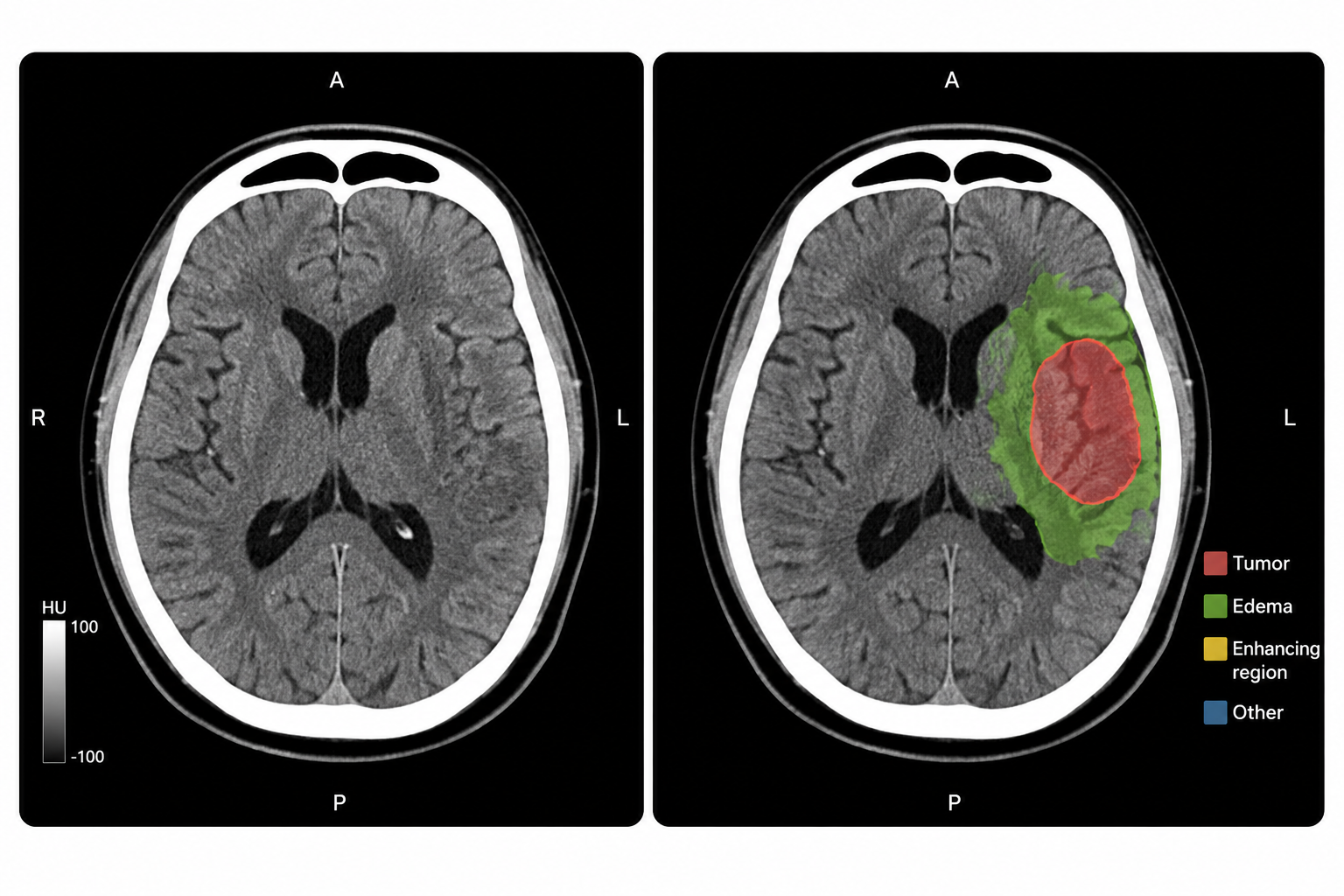
Figure 4: Input axial slice on the left alongside predicted segmentation mask overlay on the right.
04 Architecture family - what to pick
| Architecture | Encoder type | Strengths | When to use |
|---|---|---|---|
| nnU-Net ResEnc | 6-stage residual encoder + lightweight decoder | Heavier, higher-capacity encoder for better feature extraction; decoder stays cheap. Current recommended nnU-Net preset for most tasks with adequate GPU memory | Default choice when you have the GPU budget - see Section 03 |
| 3D U-Net (vanilla) | Plain convolutional, symmetric | Simple, fast, strong baseline | Small/medium datasets, limited compute |
| nnU-Net (standard plans) | Plain convolutional, auto-configured | Self-configures patch size, spacing, topology, augmentation per dataset | Default when ResEnc's extra compute isn't justified |
| UNETR | Vision Transformer + CNN decoder | Long-range context, strong on large structures | Larger datasets, complex multi-organ scenes |
| Swin UNETR | Hierarchical Swin Transformer | Sequence-to-sequence formulation with shifted-window attention for long-range dependencies | Tumors of variable shape and size, e.g. brain tumor segmentation |
For most practical engineering work, start with nnU-Net's ResEnc preset if you have the GPU memory for it - it consistently outperforms the original plain-convolution nnU-Net plans at a moderate extra compute cost, since nearly all of that extra cost goes into the encoder, which is exactly where it helps most.
05 Self-configuring networks: what nnU-Net actually does (explained simply)
This is the part people usually find confusing, so let's slow down. Forget the architecture (encoders, decoders, residual blocks) for a moment - this section is about automation, not the network shape.
In one plain sentence
"Self-configuring" means the software looks at YOUR dataset and decides, by itself, all the settings a human engineer would normally have to guess and hand-tune - things like image size, how much to shrink the scan, how to normalize brightness, and how big/deep the network should be. You don't write those settings. nnU-Net measures your data and works them out.
A simple analogy first
Think of a fully-automatic washing machine. A cheap manual machine makes you choose the water temperature, spin speed, and cycle length yourself, every time, for every load - and if you guess wrong, your clothes come out damp or your wool sweater shrinks. A smart automatic machine weighs the load, senses the fabric, and picks the settings itself. You just put the clothes in and press start.
nnU-Net is the automatic washing machine for medical image segmentation. Before it existed, a researcher had to manually pick: how big a 3D patch to feed the network, what resolution to resize scans to, how to normalize CT/MRI brightness values, how many layers the network needs, how long to train. Guess wrong, and results are poor - and there was no reliable rulebook for guessing right. nnU-Net replaced all that guesswork with automatic measurement.
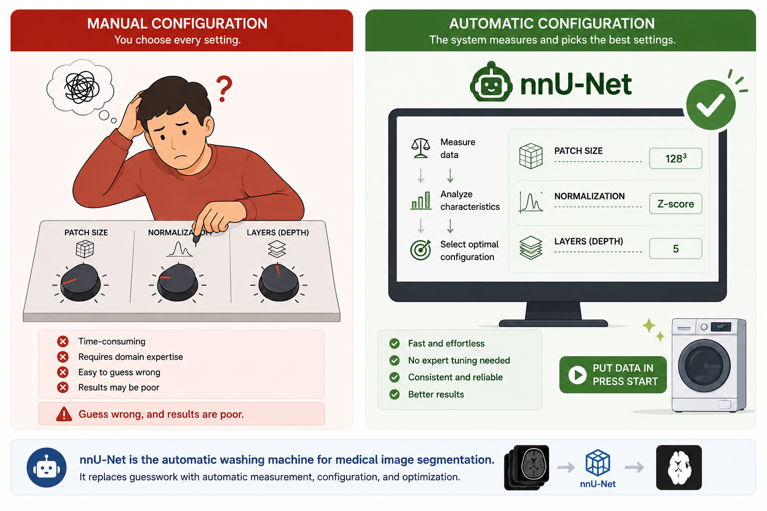
Figure 5: Manual tuning vs. automatic configuration illustration.
What exactly gets configured automatically? (with real examples)
nnU-Net looks at three things in your raw dataset before it trains anything: how the images were scanned, how big they are, and what's inside them. From that, it derives every setting below. Here are two worked examples on genuinely different datasets, so you can see the automation actually adapts rather than just using one fixed answer:
| Setting nnU-Net decides | Example A: liver CT scan, low resolution | Example B: brain MRI, high resolution |
|---|---|---|
| Target voxel spacing (how "zoomed in" the 3D grid is) | Resamples to ~1.5 x 1.5 x 2.0 mm - matches the typical spacing across the training scans | Resamples to ~1.0 x 1.0 x 1.0 mm - brain MRI needs finer detail to see small structures |
| Patch size (the 3D chunk fed to the GPU at once) | e.g. 128 x 128 x 128 voxels - liver is a large, simple shape | e.g. 160 x 192 x 128 voxels - shaped to fit the brain's proportions |
| Intensity normalization | Clip Hounsfield Units to the liver/tumor range, then z-score - CT has fixed physical units | Per-scan z-score normalization - MRI brightness has no fixed physical unit, so each scan is normalized to itself |
| Network depth / width | Fewer downsampling stages if the organ is large relative to the scan | More stages if fine detail near tissue boundaries matters |
| Batch size | Chosen so patches + network fit in the detected GPU memory | Chosen the same way - smaller if the patch size above is larger |
The exact numbers above are realistic examples, not a guarantee - nnU-Net computes the real values from your data every time, which is the whole point: nobody typed these numbers in.
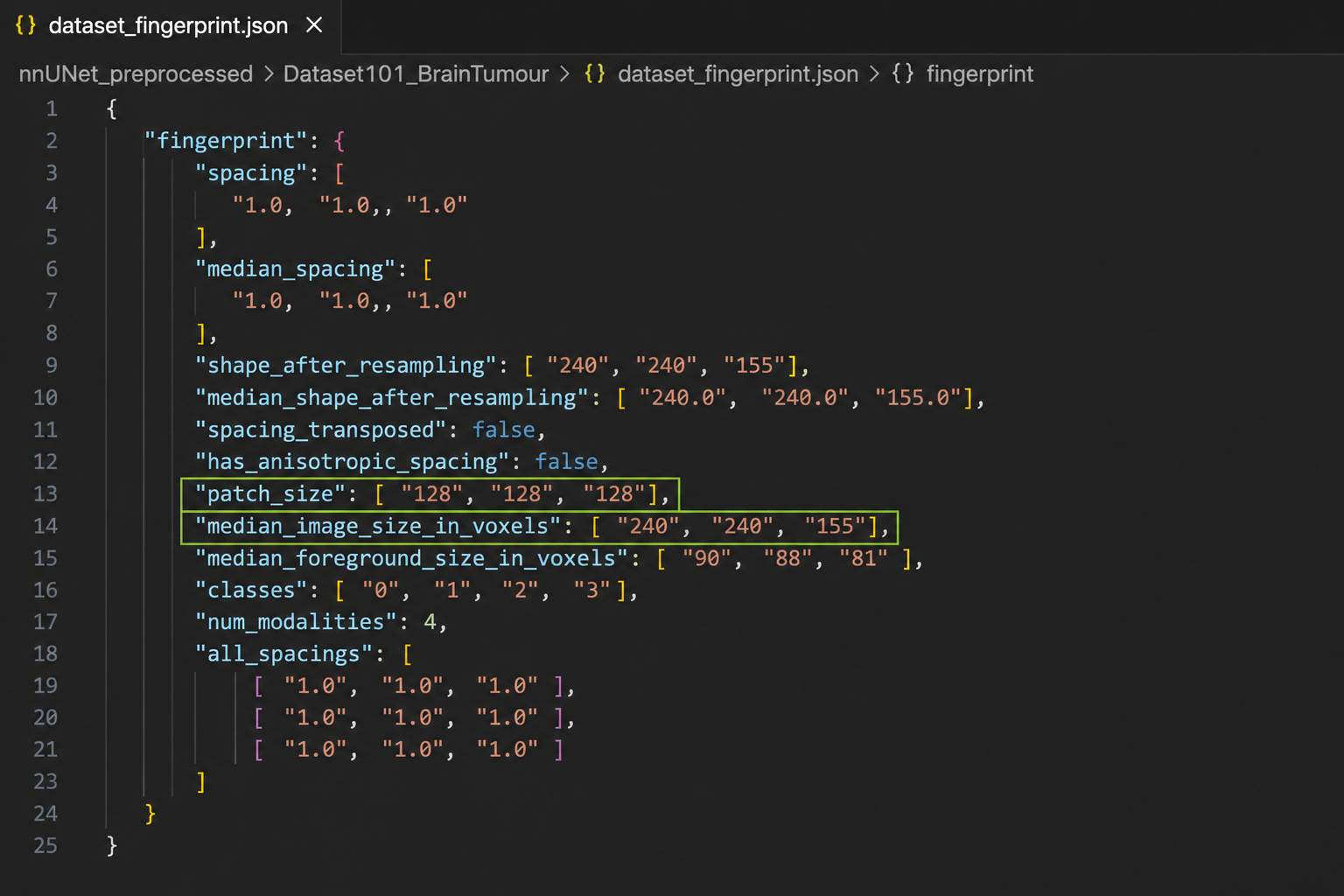
Figure 6: Generated dataset_fingerprint.json and plans.json file excerpt.
Step by step: what happens when you run nnU-Net on a new dataset
- You give it raw scans + labels. Just NIfTI files in folders - no settings, no config file to write by hand.
- It "fingerprints" the dataset. nnU-Net scans through every training case and records: image size, voxel spacing, intensity value ranges, and how much of each class (e.g. tumor vs. background) is present. Think of this like a doctor taking a patient's vitals before deciding treatment - it measures first, decides second.
- It applies fixed rules to the fingerprint. These rules were worked out by the nnU-Net authors from studying hundreds of successful segmentation pipelines, then hard-coded as heuristics (e.g. "target spacing = median spacing of the dataset", "patch size as large as fits in a given GPU budget"). This step is instant - no training needed yet.
- It generates 2-3 candidate training configurations (2D, 3D full-resolution, and sometimes a low-res + cascade pair for very large volumes) and trains each with 5-fold cross-validation.
- It compares the trained candidates and empirically picks the best - by actual validation performance, not by assumption - and can ensemble more than one if that scores even higher.
- It uses the winning configuration to run inference on new, unlabeled scans.
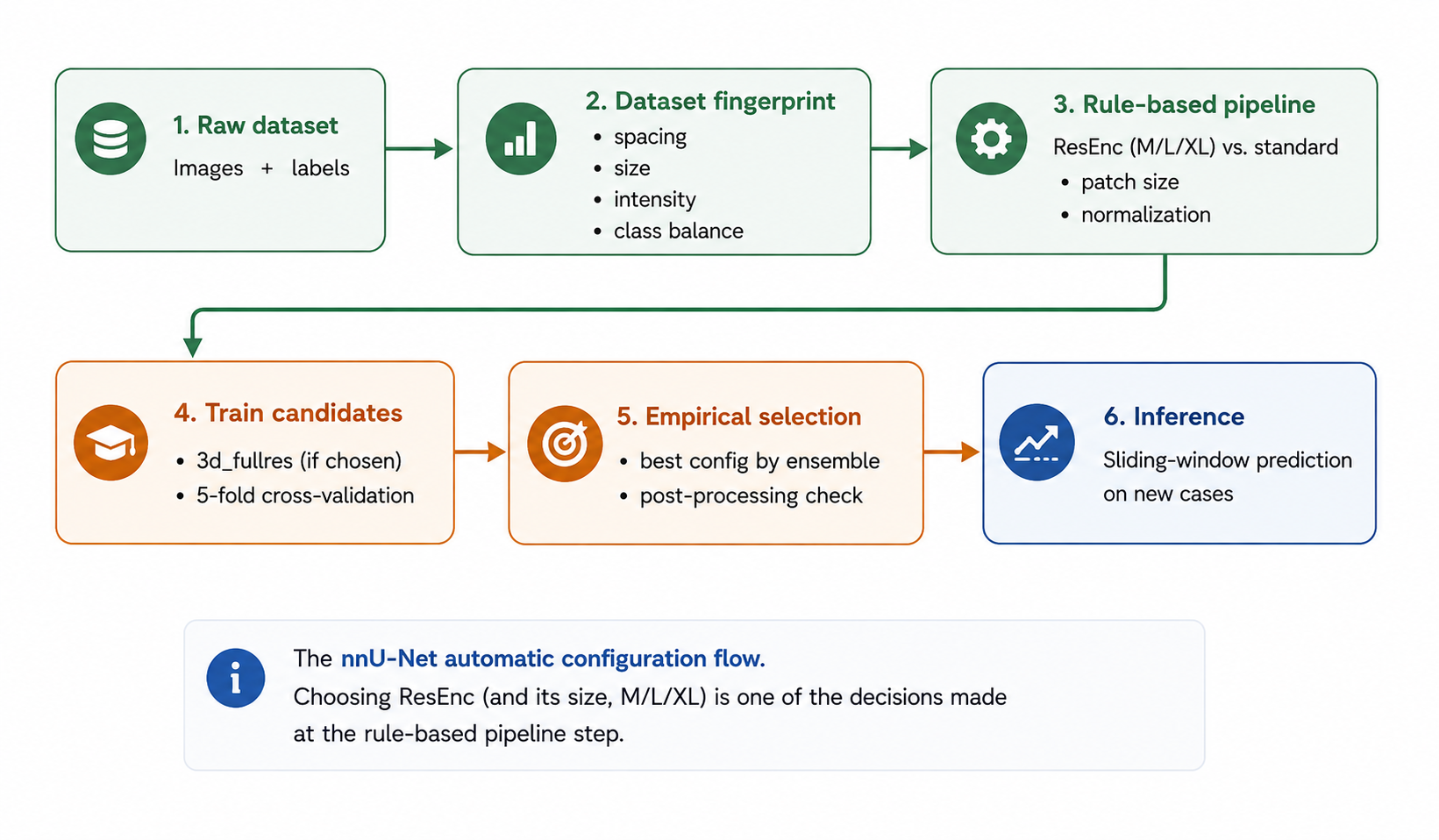
Figure 7: nnU-Net automatic configuration flow. Choosing ResEnc (and its size, M/L/XL) is one of the decisions made at the rule-based pipeline step.
Before vs. after: why this was a big deal
| Before nnU-Net (manual) | With nnU-Net (self-configuring) | |
|---|---|---|
| Patch size, spacing, normalization | Chosen by trial and error, per dataset, by an expert | Computed automatically from the dataset fingerprint |
| Network depth / width | Copied from a paper, or hand-tuned | Derived from image size and available GPU memory |
| Time to a working baseline | Days to weeks of tuning per new dataset | One command; hours to days of automatic training, no tuning |
| Reproducibility across labs | Low - every group's hand-tuned pipeline differed | High - same rules applied consistently to any dataset |
| Who can use it well | Mainly deep-learning specialists | Clinicians, students, and non-specialists can get strong results |
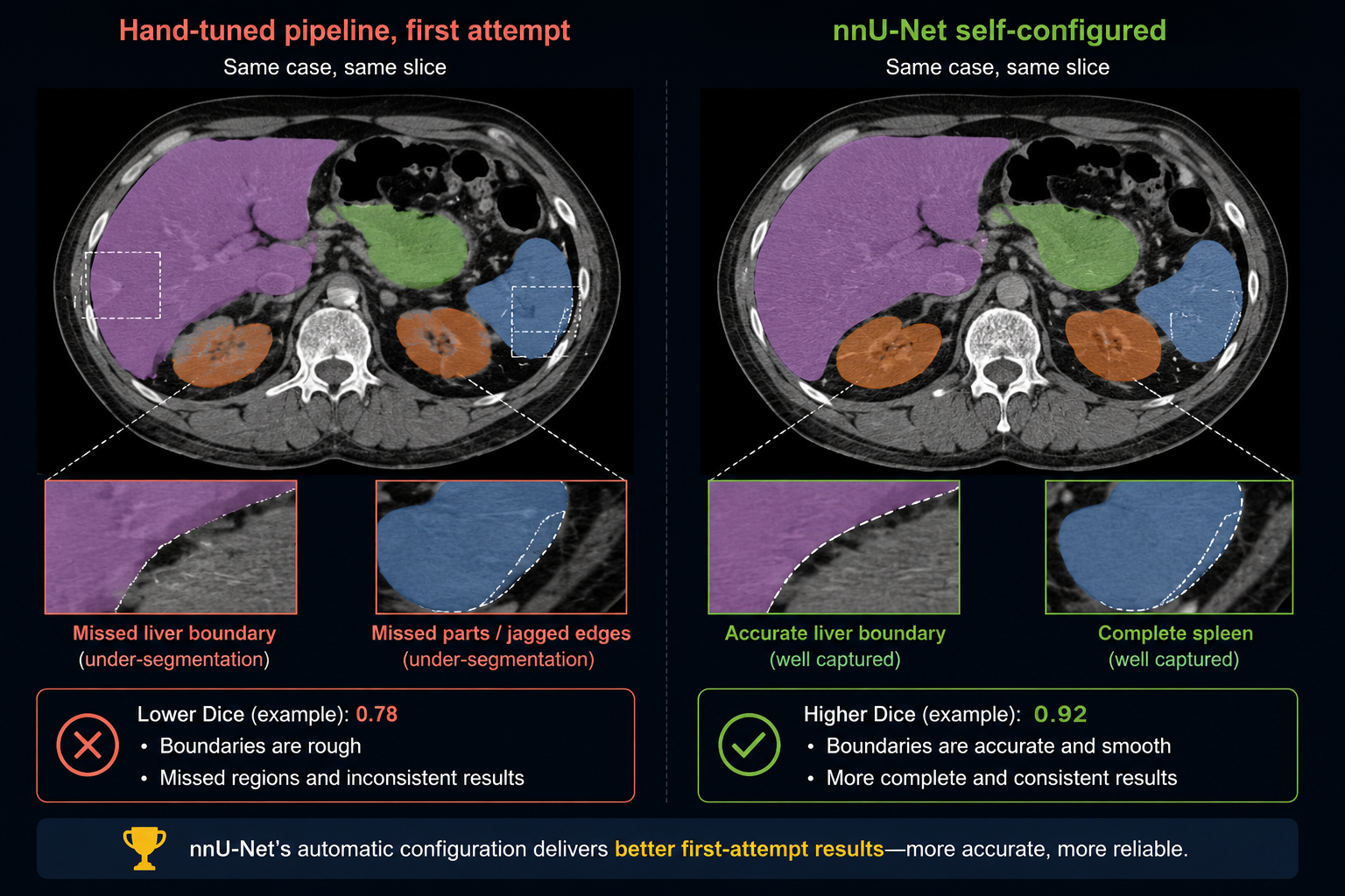
Figure 8: Hand-tuned baseline vs. nnU-Net self-configured segmentation result comparison.
Quick check: is this "AutoML"?
Close, but not quite the same thing, and this distinction trips people up:
- AutoML (in the general machine-learning sense) usually means searching over many possible architectures or hyperparameters by trial-and-error training runs, which can take enormous compute.
- nnU-Net's self-configuration is mostly rule-based, not search-based - it computes settings directly from measured dataset statistics using fixed formulas, in seconds, without training a single model. Only the final "which of 2-3 candidates wins" step (see step 4-5 above) involves actual training and comparison.
That's why nnU-Net is fast to get a strong first result from, compared to open-ended architecture search: most of its intelligence is in well-tested rules, not brute-force experimentation.
The configurations nnU-Net trains
Once the rules above have set the recipe, nnU-Net still trains a small number of different configurations and lets validation performance pick the winner, rather than assuming any one is always best:
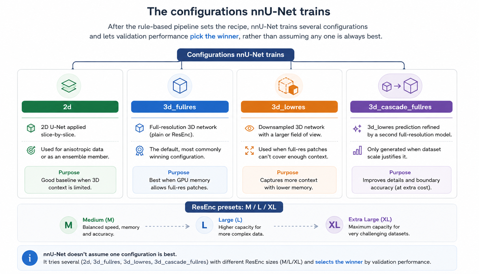
Figure 9: Overview of the 4 core configurations nnU-Net trains (2D, 3D Full-res, 3D Low-res, 3D Cascade Full-res).
ResEnc presets: M / L / XL
nnU-Net ships ResEnc at multiple capacity tiers, trading compute for accuracy - all follow the same six-stage, residual-encoder-plus-light-decoder design; they differ mainly in how many residual blocks are stacked per stage and the exact patch/batch size the planner selects for available GPU memory:
| Preset | Relative capacity | Typical GPU budget |
|---|---|---|
nnUNetResEncUNetMPlans | Medium | ~10-24 GB - close to standard nnU-Net compute cost |
nnUNetResEncUNetLPlans | Large | ~24-40 GB |
nnUNetResEncUNetXLPlans | Extra-large | 40 GB+, multi-GPU territory |
Fixed / default training parameters
Several training parameters stay fixed regardless of encoder type: learning rate 0.01, up to 1000 training epochs, a combined Cross-Entropy + Dice loss, and on-the-fly data augmentation. The "don't over-engineer what doesn't need to be engineered" philosophy is a big part of why nnU-Net generalizes so well out of the box - it spends its adaptive budget on dataset-specific decisions (like whether ResEnc is worth the extra compute for your data) rather than on things that don't need per-dataset tuning.
06 Why it works: the published evidence
This section summarizes what the primary papers actually measured, rather than just describing the architecture, so you can judge the strength of the evidence yourself and cite it accurately.
nnU-Net's original result (Isensee et al., Nature Methods, 2021)
The framework was benchmarked across 23 public datasets spanning a wide range of biomedical segmentation tasks. Using only automatic, dataset-derived configuration with no manual intervention, nnU-Net produced state-of-the-art performance and was used to win a majority of the international segmentation challenges it was entered in, at a time when nearly every other top submission relied on hand-crafted, dataset-specific pipelines. The finding motivating the whole framework was methodological: most of the field's reported gains over a vanilla U-Net came from pipeline engineering (preprocessing, patch sizing, augmentation, post-processing), not from novel network architectures.
The ResEnc scaling result (Isensee et al., MICCAI, 2024)
This later paper re-examined that claim under stricter conditions, since several newer architectures (transformer-based and, more recently, state-space/"Mamba"-based models) had since reported beating nnU-Net. The authors benchmarked CNN-based, transformer-based, and Mamba-based segmentation methods head-to-head on matched datasets, splits, and compute budgets - deliberately avoiding the common validation pitfalls (weak baselines, small test sets, ignoring compute cost) that had let earlier "new architecture beats U-Net" claims go unchallenged. Their conclusion, in the authors' own framing: state-of-the-art performance came from (1) CNN-based U-Net models, including ResNet- and ConvNeXt-style encoder variants, (2) run inside the nnU-Net framework, and (3) scaled to modern hardware - not from switching to a fundamentally different architecture family. The ResEnc M/L/XL presets are the direct output of that scaling exercise: same U-Net skeleton, heavier residual encoder, larger patch sizes, more GPU memory. In the paper's benchmarking, ResEnc variants and the related MedNeXt model consistently ranked among the strongest configurations, with ResEnc offering a favorable accuracy-for-compute trade-off versus the most expensive alternatives.
Where ResEnc tends to help the most in practice
| Dataset characteristic | Effect on ResEnc's advantage |
|---|---|
| Large training sets (hundreds+ of cases) | Larger effect - more data to exploit the extra encoder capacity |
| Fine, thin, or low-contrast structures (vessels, small lesions) | Larger effect - deeper residual features help discriminate subtle boundaries |
| Small datasets (tens of cases) | Smaller or negligible effect - standard nnU-Net plans may be equally good and cheaper |
| Severe GPU memory constraints | ResEnc may not be practical at all - see Section 08 on the M/L/XL trade-off |
This pattern is consistent with the residual encoder's core mechanism: it adds representational capacity, and capacity only pays off when there is enough signal (data, structure complexity) for the network to use it on. This is also why nnU-Net still trains and empirically compares multiple configurations rather than defaulting to the largest model - bigger isn't automatically better on every dataset.
07 Implementation guide
Two practical paths: nnU-Net's automated CLI workflow with the ResEnc preset flag for a strong baseline with minimal effort, or building the ResEnc architecture directly for custom research.
nnU-Net v2 is installed and run largely through its CLI, organized around three environment-variable-defined directories.
pip install nnunetv2

export nnUNet_raw="/data/nnUNet_raw"
export nnUNet_preprocessed="/data/nnUNet_preprocessed"
export nnUNet_results="/data/nnUNet_results"
Organize your dataset in nnU-Net's expected folder structure:
nnUNet_raw/Dataset001_LiverTumor/
├── imagesTr/
│   ├── liver_001_0000.nii.gz
│   ├── liver_002_0000.nii.gz
│   └── ...
├── labelsTr/
│   ├── liver_001.nii.gz
│   ├── liver_002.nii.gz
│   └── ...
└── dataset.json
Run fingerprint extraction and planning, requesting the ResEnc M planner explicitly:
nnUNetv2_plan_and_preprocess -d 001 --verify_dataset_integrity -pl nnUNetPlannerResEncM

# Larger capacity tiers, if you have the GPU budget:
# -pl nnUNetPlannerResEncL
# -pl nnUNetPlannerResEncXL
Train with 5-fold cross-validation, using the ResEnc plan:
nnUNetv2_train 001 3d_fullres 0 -p nnUNetResEncUNetMPlans
nnUNetv2_train 001 3d_fullres 1 -p nnUNetResEncUNetMPlans
nnUNetv2_train 001 3d_fullres 2 -p nnUNetResEncUNetMPlans
nnUNetv2_train 001 3d_fullres 3 -p nnUNetResEncUNetMPlans
nnUNetv2_train 001 3d_fullres 4 -p nnUNetResEncUNetMPlans
Find the best configuration and, if applicable, cascade/ensemble:
nnUNetv2_find_best_configuration 001 -c 3d_fullres -p nnUNetResEncUNetMPlansRun inference on new cases:
nnUNetv2_predict -i /data/imagesTs -o /data/predictions \
    -d 001 -c 3d_fullres -p nnUNetResEncUNetMPlans -f 0 1 2 3 4
The plans.json generated in step 2 records the exact per-stage block counts, patch size, and channel widths nnU-Net chose for your dataset - check it if you want the precise numbers actually used for training, since they can shift slightly from the reference [32, 64, 128, 256, 320, 320] depending on your data.
MONAI's built-in UNet class is symmetric (same block count/type on both sides), so it can't directly express an asymmetric "heavy residual encoder + light decoder" design. To build the actual ResEnc architecture in Python, use nnU-Net's own network-building package, dynamic-network-architectures, which implements exactly this class:
pip install dynamic-network-architectures torchBefore the model, set up data loading. MONAI's dictionary-style transforms handle NIfTI I/O, spacing resampling, intensity normalization, and patch sampling in one pipeline - this is the same preprocessing nnU-Net's CLI automates internally, made explicit here for a custom training loop:
import torch
from monai.data import Dataset, DataLoader, CacheDataset
from monai.transforms import (
    Compose, LoadImaged, EnsureChannelFirstd, Orientationd, Spacingd,
    ScaleIntensityRanged, CropForegroundd, RandCropByPosNegLabeld,
    RandFlipd, RandRotate90d, RandShiftIntensityd, EnsureTyped,
)

train_transforms = Compose([
    LoadImaged(keys=["image", "label"]),
    EnsureChannelFirstd(keys=["image", "label"]),
    Orientationd(keys=["image", "label"], axcodes="RAS"),
    Spacingd(keys=["image", "label"], pixdim=(1.0, 1.0, 1.0), mode=("bilinear", "nearest")),
    # CT-style intensity windowing; for MRI use NormalizeIntensityd(nonzero=True) instead
    ScaleIntensityRanged(keys=["image"], a_min=-175, a_max=250, b_min=0.0, b_max=1.0, clip=True),
    CropForegroundd(keys=["image", "label"], source_key="image"),
    RandCropByPosNegLabeld(
        keys=["image", "label"], label_key="label", spatial_size=(128, 128, 128),
        pos=2, neg=1, num_samples=2, image_key="image", image_threshold=0,
    ),
    RandFlipd(keys=["image", "label"], prob=0.5, spatial_axis=0),
    RandRotate90d(keys=["image", "label"], prob=0.3, max_k=3),
    RandShiftIntensityd(keys=["image"], offsets=0.10, prob=0.5),
    EnsureTyped(keys=["image", "label"]),
])

val_transforms = Compose([
    LoadImaged(keys=["image", "label"]),
    EnsureChannelFirstd(keys=["image", "label"]),
    Orientationd(keys=["image", "label"], axcodes="RAS"),
    Spacingd(keys=["image", "label"], pixdim=(1.0, 1.0, 1.0), mode=("bilinear", "nearest")),
    ScaleIntensityRanged(keys=["image"], a_min=-175, a_max=250, b_min=0.0, b_max=1.0, clip=True),
    CropForegroundd(keys=["image", "label"], source_key="image"),
    EnsureTyped(keys=["image", "label"]),
])

# data_dicts = [{"image": "img_001.nii.gz", "label": "lbl_001.nii.gz"}, ...]
train_ds = CacheDataset(data=train_files, transform=train_transforms, cache_rate=1.0, num_workers=4)
val_ds = Dataset(data=val_files, transform=val_transforms)

train_loader = DataLoader(train_ds, batch_size=2, shuffle=True, num_workers=4, pin_memory=True)
val_loader = DataLoader(val_ds, batch_size=1, num_workers=2)
Build a 6-stage ResEnc-style network with the feature progression from Section 03:
import torch.nn as nn
from dynamic_network_architectures.architectures.unet import ResidualEncoderUNet

model = ResidualEncoderUNet(
    input_channels=1,
    n_stages=6,
    features_per_stage=[32, 64, 128, 256, 320, 320],
    conv_op=nn.Conv3d,
    kernel_sizes=3,
    strides=[1, 2, 2, 2, 2, 2],          # stage 1 keeps full resolution
    n_blocks_per_stage=[1, 3, 4, 6, 6, 6],  # more residual blocks in deeper stages
    num_classes=2,
    n_conv_per_stage_decoder=[1, 1, 1, 1, 1],  # lightweight: 1 conv per decoder stage
    conv_bias=True,
    norm_op=nn.InstanceNorm3d,
    norm_op_kwargs={},
    dropout_op=None,
    nonlin=nn.LeakyReLU,
    nonlin_kwargs={"inplace": True},
    deep_supervision=True,
)n_blocks_per_stage above is illustrative of the "deeper stages get more blocks" pattern nnU-Net's ResEnc presets follow. For the exact values used on your dataset, always read the generated plans.json from nnUNetv2_plan_and_preprocess rather than hardcoding numbers from memory - the planner adapts these per dataset and preset size (M/L/XL).Training loop (this part is architecture-agnostic and works the same as any 3D segmentation network):
from monai.losses import DiceCELoss
from monai.metrics import DiceMetric
from monai.transforms import AsDiscrete
from monai.inferers import sliding_window_inference
from monai.data import decollate_batch
from torch.optim import SGD
from torch.amp import autocast, GradScaler

loss_function = DiceCELoss(to_onehot_y=True, softmax=True)
dice_metric = DiceMetric(include_background=False, reduction="mean")
post_pred = AsDiscrete(argmax=True, to_onehot=2)
post_label = AsDiscrete(to_onehot=2)
optimizer = SGD(model.parameters(), lr=1e-2, momentum=0.99, nesterov=True)
scaler = GradScaler()

for epoch in range(max_epochs):
    model.train()
    for batch in train_loader:
        inputs, labels = batch["image"].to(device), batch["label"].to(device)
        optimizer.zero_grad()
        with autocast("cuda"):
            outputs = model(inputs)
            loss = loss_function(outputs, labels)
        scaler.scale(loss).backward()
        scaler.step(optimizer)
        scaler.update()

    model.eval()
    with torch.no_grad():
        for val_batch in val_loader:
            val_inputs = val_batch["image"].to(device)
            val_labels = val_batch["label"].to(device)
            val_outputs = sliding_window_inference(val_inputs, (128, 128, 128), 4, model)
            val_outputs = [post_pred(i) for i in decollate_batch(val_outputs)]
            val_labels_list = [post_label(i) for i in decollate_batch(val_labels)]
            dice_metric(y_pred=val_outputs, y=val_labels_list)
    print(f"epoch {epoch} mean dice: {dice_metric.aggregate().item():.4f}")
    dice_metric.reset()
Inference on a new, unlabeled scan - sliding-window inference handles volumes larger than the training patch size by stitching overlapping predictions:
import nibabel as nib
import numpy as np

model.eval()
with torch.no_grad():
    test_data = val_transforms({"image": "new_scan.nii.gz"})
    test_input = test_data["image"].unsqueeze(0).to(device)
    logits = sliding_window_inference(test_input, (128, 128, 128), 4, model, overlap=0.5)
    pred_mask = torch.argmax(logits, dim=1)[0].cpu().numpy().astype(np.uint8)

    # write the predicted mask back out as a NIfTI file, reusing the input affine
    ref = nib.load("new_scan.nii.gz")
    nib.save(nib.Nifti1Image(pred_mask, affine=ref.affine), "new_scan_pred.nii.gz")
Understanding ResEnc is easier after implementing a plain 3D U-Net by hand. This is a minimal, dependency-light (pure PyTorch) implementation of the original Çiçek et al. 3D U-Net design - a symmetric encoder/decoder with plain (non-residual) convolutional blocks. Compare this against the ResEnc block diagram in Section 03: the only structural difference ResEnc adds is the identity/projection skip inside each encoder block.
import torch
import torch.nn as nn

class ConvBlock(nn.Module):
    """Two 3x3x3 convolutions, each followed by instance norm + LeakyReLU."""
    def __init__(self, in_ch, out_ch):
        super().__init__()
        self.block = nn.Sequential(
            nn.Conv3d(in_ch, out_ch, kernel_size=3, padding=1, bias=False),
            nn.InstanceNorm3d(out_ch, affine=True),
            nn.LeakyReLU(negative_slope=0.01, inplace=True),
            nn.Conv3d(out_ch, out_ch, kernel_size=3, padding=1, bias=False),
            nn.InstanceNorm3d(out_ch, affine=True),
            nn.LeakyReLU(negative_slope=0.01, inplace=True),
        )
    def forward(self, x):
        return self.block(x)

class Down(nn.Module):
    """Strided conv downsample, then a ConvBlock (plain nnU-Net uses strided conv, not max-pool)."""
    def __init__(self, in_ch, out_ch):
        super().__init__()
        self.downsample = nn.Conv3d(in_ch, in_ch, kernel_size=2, stride=2)
        self.conv = ConvBlock(in_ch, out_ch)
    def forward(self, x):
        return self.conv(self.downsample(x))

class Up(nn.Module):
    """Transposed-conv upsample, concatenate the skip connection, then a ConvBlock."""
    def __init__(self, in_ch, skip_ch, out_ch):
        super().__init__()
        self.upsample = nn.ConvTranspose3d(in_ch, in_ch, kernel_size=2, stride=2)
        self.conv = ConvBlock(in_ch + skip_ch, out_ch)
    def forward(self, x, skip):
        x = self.upsample(x)
        x = torch.cat([x, skip], dim=1)   # the skip connection: encoder detail + decoder context
        return self.conv(x)

class PlainUNet3D(nn.Module):
    """A 5-stage plain 3D U-Net, matching the Cicek et al. (2016) design."""
    def __init__(self, in_channels=1, num_classes=2, features=(32, 64, 128, 256, 320)):
        super().__init__()
        f1, f2, f3, f4, f5 = features
        self.stem = ConvBlock(in_channels, f1)          # stage 1: full resolution
        self.enc2 = Down(f1, f2)                         # stage 2
        self.enc3 = Down(f2, f3)                         # stage 3
        self.enc4 = Down(f3, f4)                         # stage 4
        self.bottleneck = Down(f4, f5)                   # stage 5: bottleneck

        self.dec4 = Up(f5, f4, f4)
        self.dec3 = Up(f4, f3, f3)
        self.dec2 = Up(f3, f2, f2)
        self.dec1 = Up(f2, f1, f1)

        self.seg_head = nn.Conv3d(f1, num_classes, kernel_size=1)   # 1x1x1 conv to class logits

    def forward(self, x):
        s1 = self.stem(x)          # full resolution
        s2 = self.enc2(s1)
        s3 = self.enc3(s2)
        s4 = self.enc4(s3)
        b  = self.bottleneck(s4)   # deepest / smallest resolution

        d4 = self.dec4(b, s4)
        d3 = self.dec3(d4, s3)
        d2 = self.dec2(d3, s2)
        d1 = self.dec1(d2, s1)
        return self.seg_head(d1)   # logits, shape [B, num_classes, D, H, W]

if __name__ == "__main__":
    model = PlainUNet3D(in_channels=1, num_classes=3)
    x = torch.randn(1, 1, 128, 128, 128)   # [batch, channels, D, H, W]
    out = model(x)
    print(out.shape)   # torch.Size([1, 3, 128, 128, 128])
print(sum(p.numel() for p in model.parameters()), "parameters")ConvBlock inside each encoder stage with a residual version that adds its input back before the final activation (see Section 03's block diagram), (2) stack more than one such block per encoder stage, increasingly so with depth, (3) keep the decoder's ConvBlock as a single plain convolution rather than two. That's the entire structural delta between this plain network and the production ResidualEncoderUNet shown in the previous tab - useful to implement once yourself so the architecture in Section 03 isn't just a diagram.A minimal loss function and single training step, using only PyTorch (no MONAI), to make the forward/backward mechanics explicit:
import torch.nn.functional as F

def dice_ce_loss(logits, target, num_classes, eps=1e-5):
    """Combined soft-Dice + cross-entropy loss, the nnU-Net default."""
    ce = F.cross_entropy(logits, target)

    probs = F.softmax(logits, dim=1)
    target_onehot = F.one_hot(target, num_classes).permute(0, 4, 1, 2, 3).float()
    dims = (0, 2, 3, 4)
    intersection = torch.sum(probs * target_onehot, dims)
    union = torch.sum(probs + target_onehot, dims)
    dice = (2.0 * intersection + eps) / (union + eps)
    dice_loss = 1.0 - dice.mean()

    return ce + dice_loss

def train_step(model, optimizer, image, label, num_classes):
    model.train()
    optimizer.zero_grad()
    logits = model(image)                       # [B, C, D, H, W]
    loss = dice_ce_loss(logits, label, num_classes)  # label: [B, D, H, W], integer class ids
    loss.backward()
    optimizer.step()
    return loss.item()
08 Practical engineering tips
- ResEnc needs more GPU memory than plain nnU-Net. Budget for it explicitly - drop to the M preset (or standard nnU-Net plans) rather than shrinking patch size drastically, since patch size matters a lot for segmentation quality.
- Patch-based training is mandatory. Full CT/MRI volumes rarely fit in GPU memory at full resolution - train on random patches and run sliding-window inference at test time.
- Class imbalance: oversample foreground-containing patches, and prefer Dice + Cross-Entropy compound losses over plain cross-entropy.
- Normalize intensities per modality. CT: clip Hounsfield Units to the relevant tissue range and z-score using dataset-wide foreground statistics. MRI: per-image z-score, since MRI has no fixed physical intensity unit.
- Resample to consistent voxel spacing before training - inconsistent spacing across scanners/institutions is one of the most common silent causes of poor generalization. This is exactly what nnU-Net's fingerprinting step automates.
- Keep the decoder light on purpose. Don't be tempted to add residual blocks to the decoder too - the whole point of this design is spending capacity where it helps most (the encoder), and a heavier decoder mostly just adds compute without proportional accuracy gains.
- Deep supervision helps ResEnc converge - auxiliary losses at intermediate decoder resolutions are standard in nnU-Net's ResEnc presets and meaningfully speed up training.
- Mixed precision is essential for 3D volumes - full FP32 training is 2-3x slower and often won't fit on consumer GPUs.
- 5-fold cross-validation, not a single split - medical datasets are usually small enough that one split gives a noisy performance estimate.
09 Evaluation metrics
| Metric | What it measures | Notes |
|---|---|---|
| Dice similarity coefficient | Volumetric overlap | Standard primary metric - report per-class and mean |
| Hausdorff distance (95th pct.) | Worst-case boundary error | Complements Dice, which can look good with a locally bad boundary |
| Sensitivity / specificity | Voxel/lesion-level detection accuracy | Important for screening/detection, not just delineation |
| Volumetric error | Predicted vs. true structure volume | Clinically meaningful for tumor burden, organ atrophy |
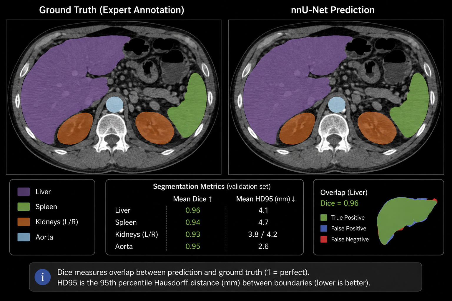
Figure 10: Ground-truth expert mask vs. model predicted segmentation mask.
Always evaluate with proper cross-validation and, ideally, an external/held-out institutional test set - performance on the training distribution alone systematically overstates real-world generalization.
10 Toolbox summary
| nnunetv2 | Self-configuring 3D segmentation, including the ResEnc presets |
| dynamic-network-architectures | The actual ResidualEncoderUNet implementation used by nnU-Net |
| MONAI / NiBabel / SimpleITK | 3D volume I/O, preprocessing, augmentation |
| MONAI UNETR / SwinUNETR | Transformer-based 3D segmentation alternative |
| Weights & Biases / MLflow | Experiment tracking |
| Decathlon / AMOS / BTCV | Benchmark datasets |
11 References
Primary sources first (in the order the ideas build on each other), followed by benchmark datasets and software. Each entry notes why it's relevant to this guide.
Core architecture papers
| Citation | Why it matters here |
|---|---|
| Ronneberger, O., Fischer, P., Brox, T. U-Net: Convolutional Networks for Biomedical Image Segmentation. MICCAI 2015. arXiv:1505.04597 | Origin of the encoder-decoder-plus-skip-connections design (Section 00, 02). |
| Çiçek, Ö., Abdulkadir, A., Lienkamp, S.S., Brox, T., Ronneberger, O. 3D U-Net: Learning Dense Volumetric Segmentation from Sparse Annotation. MICCAI 2016. | Extends every 2D op to 3D, the direct ancestor of the volumetric network in this guide (Section 00, 01). |
| He, K., Zhang, X., Ren, S., Sun, J. Deep Residual Learning for Image Recognition. CVPR 2016. | Source of the residual-block design (skip-add before final activation) used in every ResEnc encoder stage (Section 03). |
| Isensee, F., Petersen, J., Klein, A. et al. nnU-Net: Self-adapting Framework for U-Net-Based Medical Image Segmentation. arXiv 2018. arXiv:1809.10486 | First description of the self-configuring pipeline, pre-dating the journal version (Section 00, 05). |
| Isensee, F., Jaeger, P.F., Kohl, S.A.A., Petersen, J., Maier-Hein, K.H. nnU-Net: a self-configuring method for deep learning-based biomedical image segmentation. Nature Methods 18, 203-211 (2021). | The formal, widely-cited result: automatic configuration wins the majority of benchmark challenges entered, with no manual tuning (Section 06). |
| Isensee, F.*, Wald, T.*, Ulrich, C.*, Baumgartner, M.*, Roy, S., Maier-Hein, K.†, Jäger, P.F.† nnU-Net Revisited: A Call for Rigorous Validation in 3D Medical Image Segmentation. MICCAI 2024. arXiv:2404.09556 | Introduces the ResEnc M/L/XL presets and the rigorous CNN-vs-transformer-vs-Mamba benchmark this guide's Section 06 summarizes. Cite this paper specifically when using the ResEnc presets. |
Related architectures mentioned in Section 04
- Hatamizadeh, A. et al. UNETR: Transformers for 3D Medical Image Segmentation. WACV 2022.
- Hatamizadeh, A. et al. Swin UNETR: Swin Transformers for Semantic Segmentation of Brain Tumors in MRI Images. BrainLes / MICCAI Workshop 2022.
- Roy, S. et al. MedNeXt: Transformer-driven Scaling of ConvNets for Medical Image Segmentation. MICCAI 2023. - the ConvNeXt-style CNN that performs comparably to ResEnc in the 2024 benchmark.
Benchmark datasets used to evaluate these methods
- Medical Segmentation Decathlon (MSD) - 10 multi-organ, multi-modality tasks, a standard nnU-Net benchmark.
- KiTS19 / KiTS23 - kidney and kidney tumor segmentation challenge, where ResEnc was first introduced internally at DKFZ.
- AMOS22 - large-scale abdominal multi-organ CT/MRI benchmark.
- BTCV (Beyond the Cranial Vault) - multi-atlas abdominal CT labeling challenge.
- BraTS (Brain Tumor Segmentation) - annual MICCAI challenge for glioma segmentation in MRI.
Software
- MIC-DKFZ/nnUNet - reference implementation, CLI, and the
resenc_presets.mddocumentation used in Section 07. - MIC-DKFZ/dynamic-network-architectures - the
ResidualEncoderUNetclass used directly in Section 07's code. - Project MONAI - medical-imaging-specific PyTorch library for I/O, transforms, losses, metrics, and inference used throughout Section 07.
- arXiv.org - open-access preprint host for most papers above; search by title if a DOI link is unavailable to you.
plans.json for the values actually used in training, and cite the 2024 MICCAI paper (not just the 2021 Nature Methods paper) when you use the ResEnc presets specifically.